TL;DR — The Cpk normality assumption isn't a soft approximation — it's a specific function evaluation. The KS test measures the supremum distance between your empirical CDF and the Gaussian CDF. When it rejects, it's not a technicality — it's a proof that the mapping from σ to tail probability (which is the entire basis of Cpk) is invalid for your data. Chebyshev's inequality gives you the worst-case bound on what ±kσ actually covers for arbitrary distributions. The gap between the Gaussian promise and the Chebyshev guarantee is where your unreported defects live.
This is Part 3 of the Cpk normality assumption series. Parts and covered the business case. This one covers the math.
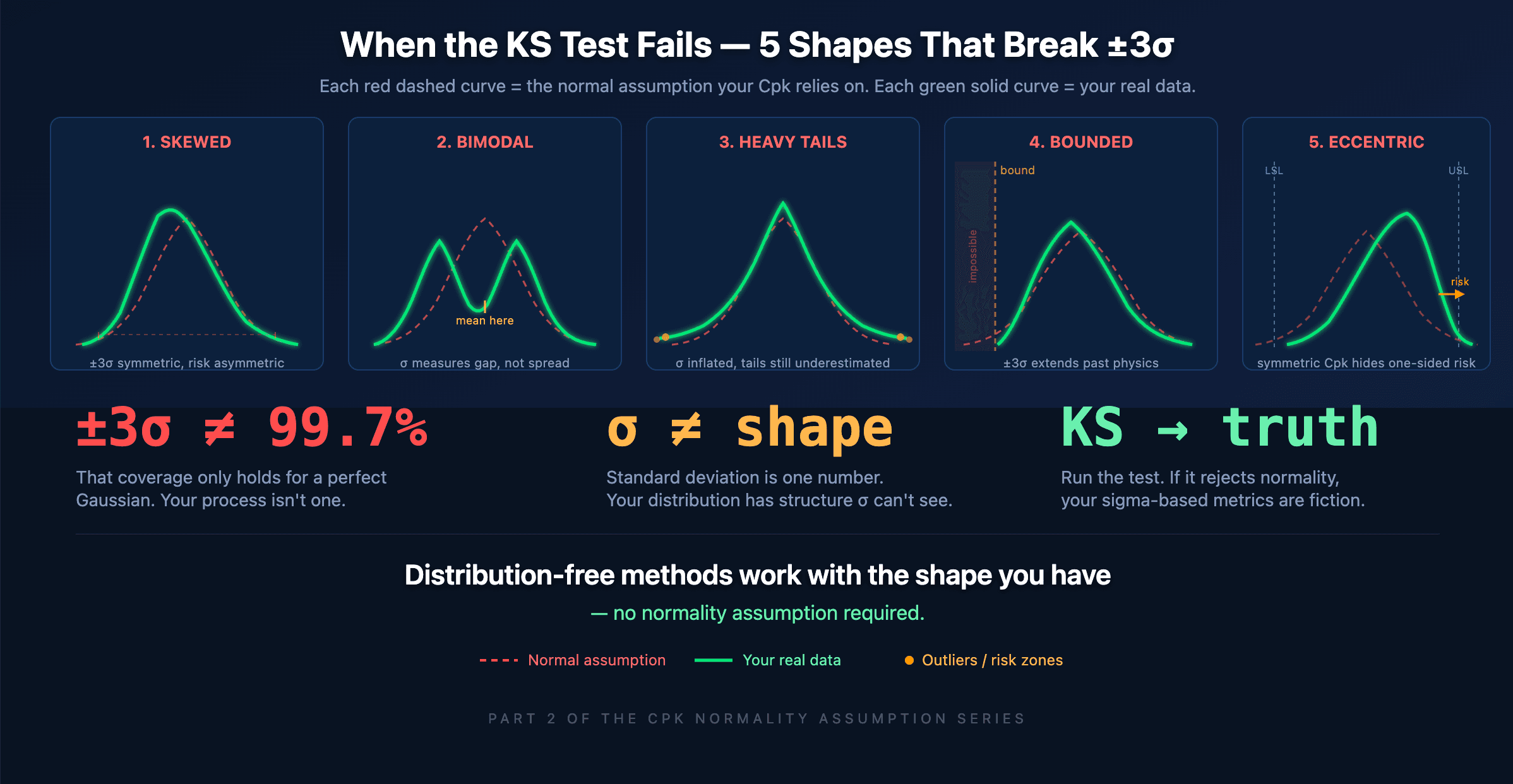
When a KS test rejects the Cpk normality assumption, the ±3σ interval stops meaning 99.7%. Here are five real process shapes where sigma-based reasoning falls apart — and what your data is actually telling you.
This looks like a simple ratio. But the interpretive leap from Cpk to defect rate depends entirely on a specific function — the Gaussian survival function:
P(X > USL) = 1 − Φ((USL − μ) / σ)
where Φ is the standard normal CDF. When we say Cpk = 1.33 corresponds to 63 ppm defect rate, we are computing 1 − Φ(4) on each tail. The function Φ is the CDF of exactly one distribution: N(μ, σ²). If the true distribution F of your process data is not Gaussian, then Φ is the wrong function, and every ppm number derived from Cpk is a non-sequitur.
This is not an approximation concern. It's a category error. We are evaluating the wrong function.
The Kolmogorov–Smirnov Statistic: Measuring How Wrong Φ Is
Andrey Kolmogorov (1933) and Nikolai Smirnov (1948) gave us a precise tool to quantify the departure of empirical data from a hypothesized distribution.
Given n observations x₁, ..., xₙ, define the empirical CDF:
Fₙ(x) = (1/n) · #{i : xᵢ ≤ x}
The KS statistic is the supremum of the absolute difference between Fₙ and the hypothesized CDF F₀ (in our case, the Gaussian Φ with parameters estimated from the data):
Dₙ = sup_x |Fₙ(x) − F₀(x)|
This is a uniform metric on the space of distribution functions. It captures the single worst-case point of departure — the value of x where your data's CDF diverges most from the Gaussian hypothesis.
Kolmogorov proved that under the null hypothesis (data truly drawn from F₀), the rescaled statistic √n · Dₙ converges in distribution to the Kolmogorov distribution K:
This gives us exact critical values. When √n · Dₙ exceeds the critical threshold for significance level α, we reject the null. The test is consistent — for any true distribution F ≠ F₀, the probability of rejection converges to 1 as n → ∞.
What This Means for Your Factory
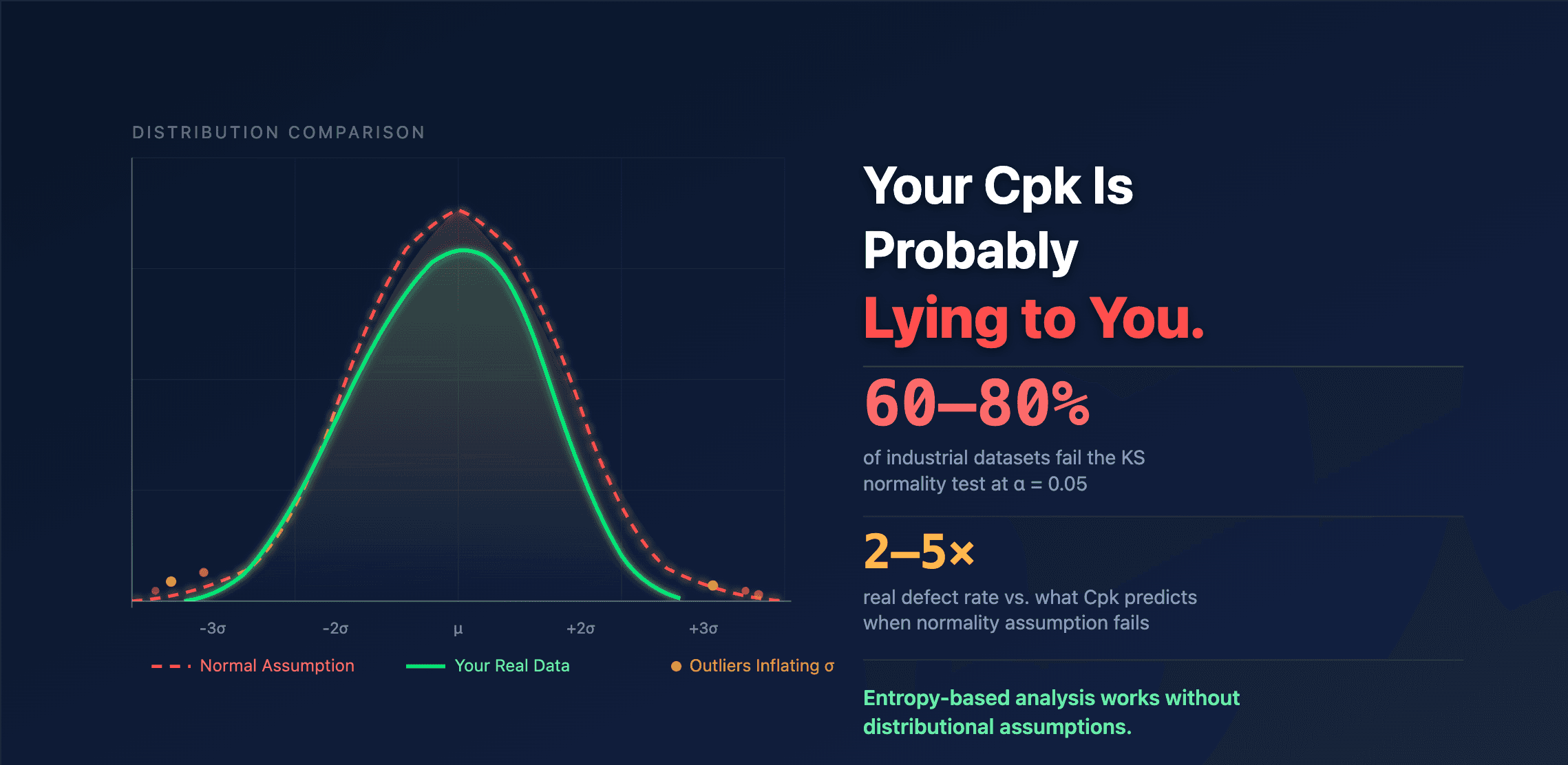
When the KS test rejects at α = 0.05 with p < 0.01 — which happens for 60–80% of industrial datasets — it is telling you:
The supremum distance Dₙ between your empirical CDF and the Gaussian CDF is too large to have arisen by sampling noise. The deviation is real. And because Dₙ measures the worst-case point, the rejection identifies the region of x where Fₙ(x) and Φ(x) disagree most — which is almost always in the tails. Exactly where your out-of-spec probability lives.
Chebyshev's Inequality: The Honest Bound
Pafnuty Chebyshev (1867) proved what is arguably the most important inequality in applied statistics. For any random variable X with finite mean μ and finite variance σ²:
P(|X − μ| ≥ kσ) ≤ 1/k²
No distributional assumption. No shape requirement. Just finite first and second moments.
Compare the Gaussian promise to the Chebyshev guarantee:
Interval
Gaussian coverage
Chebyshev worst-case coverage
±1σ
68.27%
≥ 0% (trivial bound)
±2σ
95.45%
≥ 75.00%
±3σ
99.73%
≥ 88.89%
±4σ
99.994%
≥ 93.75%
±6σ (Six Sigma)
99.9999998%
≥ 97.22%
Read that table carefully. When you report ±3σ covers 99.73% of your process, you are using the Gaussian column. But if the KS test rejected normality, you have no right to that column. The only universal guarantee is Chebyshev's: ±3σ covers at least 88.89%.
The gap is enormous. At ±3σ, the Gaussian predicts 2,700 ppm outside the interval. Chebyshev allows up to 111,111 ppm. Your real process is somewhere in between — and without knowing the true distribution shape, you can't say where.
For Six Sigma: the Gaussian promise is 3.4 defects per billion (after the 1.5σ shift convention) or 2 ppb without shift. Chebyshev says: at most 27,778 ppm. That's a factor of 8 million between the optimistic and pessimistic bounds. Your Cpk lives in this chasm, pretending the Gaussian column applies.
The Glivenko–Cantelli Bridge: Why More Data Doesn't Save You
One common objection: "With enough data, the empirical CDF converges to the true CDF anyway, so does it matter?"
The Glivenko–Cantelli theorem (1933) states:
sup_x |Fₙ(x) − F(x)| → 0 almost surely as n → ∞
where F is the true distribution. This is correct and fundamental. The empirical CDF does converge uniformly to the truth. But this theorem helps you only if you use Fₙ directly. The moment you replace Fₙ with Φ (the Gaussian approximation) to compute tail probabilities, you're discarding the very convergence that Glivenko–Cantelli guarantees.
In other words: your data is converging to the truth. Your Cpk formula is not using the truth. It's using Φ. And the KS test just told you Φ is wrong.
The Quantitative Damage: Taylor-Expanding the Error
Let F be the true CDF and Φ the Gaussian CDF with matched mean and variance. The error in the tail probability estimate at the upper spec limit is:
ΔP = F(USL) − Φ((USL − μ) / σ)
For mildly non-normal distributions, we can approximate F using an Edgeworth expansion:
where γ₁ is skewness, γ₂ is excess kurtosis, and φ is the standard normal PDF. The key insight: the correction terms are multiplied by φ(x), which is small in the body but the polynomial prefactors (x² − 1), (x³ − 3x) grow large in the tails. So even modest skewness (γ₁ = 0.5) or excess kurtosis (γ₂ = 2) can cause the tail probability to differ from the Gaussian estimate by a factor of 2–10× at the ±3σ point.
Industrial data commonly shows γ₁ in the range 0.3–1.5 and γ₂ in the range 1–6. At these values, the Edgeworth correction at ±3σ is not a small perturbation — it's a dominant term. The Gaussian tail estimate is not slightly off. It's structurally wrong.
Why Cpk Normality Assumption Failure Is Not a Rounding Error
Assembling the pieces:
Kolmogorov–Smirnov tells you the hypothesis F = Φ is rejected. The departure is statistically significant and concentrated in a specific region of x (typically the tails).
Chebyshev tells you the worst case. Without distributional knowledge, ±3σ guarantees only 88.89% coverage, not 99.73%. The gap is a factor of 41× in tail probability.
Edgeworth tells you the typical case. For realistic industrial skewness and kurtosis values, tail probabilities are 2–10× higher than Gaussian predictions.
Glivenko–Cantelli tells you the data knows the truth. The empirical CDF converges to the real distribution. But Cpk doesn't use the empirical CDF — it uses Φ, which was just rejected.
The Cpk normality assumption is not an approximation that degrades gracefully. It's a function evaluation on the wrong function. When the KS test rejects, it is telling you — with quantifiable confidence — that the function your entire quality reporting framework is built on does not describe your process.
The Distribution-Free Alternative
The mathematical answer is straightforward: use the empirical distribution directly.
The empirical CDF Fₙ is the nonparametric maximum likelihood estimator of F. By Glivenko–Cantelli, it converges uniformly. By the Dvoretzky–Kiefer–Wolfowitz inequality (1956):
P(sup_x |Fₙ(x) − F(x)| > ε) ≤ 2 · exp(−2nε²)
This gives finite-sample confidence bands around Fₙ without any distributional assumption. You can compute P(X > USL) directly from Fₙ and bound the estimation error explicitly. No Φ required. No normality assumption. No Cpk fiction.
Entropy-based methods go further: they derive robust estimates of location, scale, and support bounds using influence functions that are bounded by construction. This makes them resistant to the outliers and contamination that plague industrial datasets — the same outliers that inflate σ and distort every sigma-based metric.
The mathematics has been available since the 1930s. The computational tools to apply it routinely have been available for a decade. The only thing keeping ±kσ intervals and Gaussian-dependent Cpk in place is institutional inertia.
The Takeaway
The KS test is not a bureaucratic checkbox. It is a hypothesis test with known convergence properties, exact critical values, and a clear interpretation: the supremum distance between your data and the Gaussian model exceeds what sampling noise can explain. When it rejects, Chebyshev's inequality defines the honest bound on what your σ-based intervals actually cover. The Edgeworth expansion quantifies how far off your tail estimates are. And Glivenko–Cantelli guarantees that the empirical distribution — which your Cpk formula ignores — is converging to the truth.
The Cpk normality assumption is not a minor technicality. It is the load-bearing wall of your entire quality metric framework. The KS test is telling you it has cracked. The question is whether you keep decorating the room or inspect the foundation.