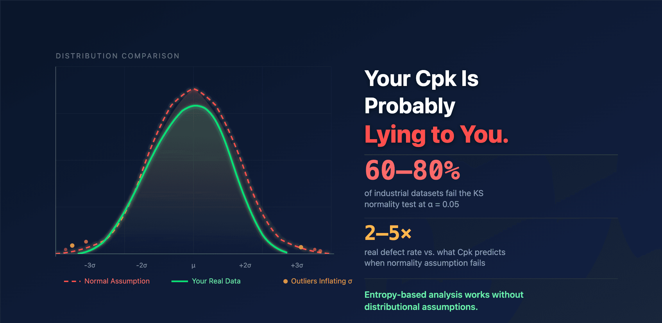
In the previous article about cpk normality assumption, we established that 60–80% of industrial datasets fail the Kolmogorov-Smirnov normality test. The Cpk normality assumption doesn't hold for most real processes.
But what does that actually mean in practice? When the KS test rejects normality, it's telling you that your data's shape deviates from the Gaussian bell curve. The ±1σ = 68%, ±2σ = 95%, ±3σ = 99.7% rules are properties of that specific shape. Once the shape changes, those percentages become meaningless — and the direction of the error depends on how the shape changes.
The mathematical proof that your Cpk is wrong: Kolmogorov–Smirnov convergence, Chebyshev’s inequality, and why σ-based intervals fail when the empirical CDF diverges from the Gaussian hypothesis. A master’s-level walkthrough of what the Cpk normality assumption actually assumes — and where it breaks
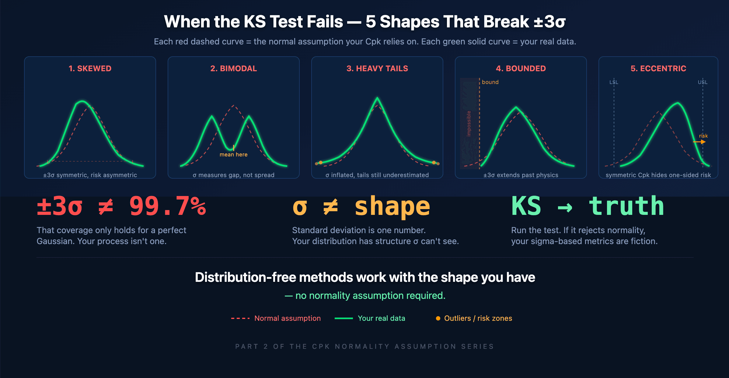
Here are five common process shapes where sigma-based reasoning breaks down, what each one does to your intervals, and what it means for your quality decisions.
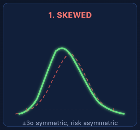
Case 1: Skewed Distribution — ±3σ Points the Wrong Way
A machining process cutting close to a physical hard stop. Surface roughness values that can't go below zero. Chemical concentrations approaching a saturation limit. All of these produce skewed data — a long tail on one side and a short tail on the other.
The ±3σ interval is always symmetric around the mean. For skewed data, this creates a fundamental mismatch: the interval extends too far on the short-tail side (wasting tolerance budget on defects that can't happen) and not far enough on the long-tail side (underestimating the risk where it actually lives).
A right-skewed process with mean = 50, σ = 2, and spec limits at 44–56 gives you a reassuring Cpk of 1.0. But the real distribution puts 2% of parts above 56 and only 0.01% below 44. The symmetric ±3σ interval says the risk is equal on both sides. It's off by a factor of 200 on the high side. Your scrap bin knows which side the rejects come from. Your Cpk report doesn't.
Case 2: Bimodal Distribution — σ Averages Between Two Processes
Two mold cavities producing slightly different dimensions. Day shift and night shift with different thermal conditions. Two raw material suppliers with different lot properties. When these sub-populations mix in your dataset, you get a bimodal distribution — two peaks with a valley between them.
Standard deviation calculated on bimodal data produces a number that doesn't describe either population. It describes the gap between them. The mean lands in the valley where almost no actual parts exist, and ±3σ extends outward to cover both peaks plus their tails. The result is a massively inflated interval that tells you nothing about what either sub-process is actually doing.
Consider two cavity populations centered at 49.8 and 50.4 mm, each with internal σ of 0.15 mm. Pooled together, the calculated σ jumps to 0.45 mm — three times the real variability of either cavity. Your Cpk drops from a comfortable 2.2 (per cavity) to a marginal 0.74 (pooled). A quality engineer looking at the pooled number would flag the process for improvement. In reality, both cavities are individually excellent. The "problem" is that you're computing a single σ across two distinct populations. The fix isn't tighter control — it's recognizing that you have two processes, not one.
Case 3: Heavy Tails — More Outliers Than σ Predicts
A normal distribution predicts that values beyond ±3σ occur 0.3% of the time — roughly 3 parts in 1,000. Many industrial processes produce outliers at rates of 1–5%, sometimes more. Measurement noise, transient equipment hiccups, contaminated raw material lots, and startup effects all generate occasional extreme values that a Gaussian tail doesn't account for.
When you compute σ on heavy-tailed data, the outliers inflate it. Now your ±3σ interval is wider than it should be for the core process, but still not wide enough to capture the true tail behavior. You end up in the worst of both worlds: the interval is too wide to be useful as a process capability description (making your process look less capable than it is), and simultaneously too narrow to predict the actual frequency of extreme events.
This is the scenario where the Cpk normality assumption most dangerously misleads. A Cpk of 1.33 on heavy-tailed data might imply a defect rate of 63 ppm. The real rate, driven by the fat tails, could be 500 ppm or more. The factor-of-eight gap between predicted and actual defects shows up in warranty claims, customer complaints, and sorting costs — but never in the capability report.
Case 4: Bounded and Truncated Data — σ Extends Past Physical Limits
If your process measures a percentage (0–100%), a concentration (≥ 0), a surface roughness (≥ 0), or any physical quantity with hard limits, the ±3σ interval can extend into regions that are physically impossible. A concentration with mean = 2 ppm and σ = 1.5 ppm gives a lower 3σ limit of −2.5 ppm. Negative concentration doesn't exist.
Truncated data creates a subtler version of the same problem. If your inline measurement system has an automatic sort that removes parts outside specification, the remaining data is clipped. Computing σ on clipped data underestimates the true process spread. Your Cpk looks better than reality because the evidence of non-conformance was physically removed before the calculation.
Both cases violate the same core of the Cpk normality assumption: the Gaussian distribution extends from −∞ to +∞, and σ-based intervals inherit that property. Real processes have boundaries. When your measurement sits near one, symmetric intervals become nonsensical — and the tail probability calculations behind Cpk become fiction.
Case 5: Eccentric Process Center — The Mean Isn't Where It Matters
Tool wear causes a progressive drift during a production run. A process targets the low end of the spec window to maximize tool life. Asymmetric adjustment after changeover. All of these produce data where the mean sits off-center relative to the spec limits, and the distribution is asymmetric around that mean.
The ±3σ interval, being symmetric, allocates equal margin on both sides of the mean. But the process doesn't use that margin equally. If the mean is shifted toward the upper spec limit and the distribution has a longer tail in the same direction, the real out-of-spec risk on the high side can be 10× or 50× what the symmetric Cpk formula predicts. Meanwhile, the low side has massive unused margin that the symmetric interval "reserves" but the process never needs.
An asymmetric process centered at 50.3 in a 48–52 spec window, with the long tail pointing toward 52, might show a balanced Cpk of 1.1. Decompose it: Cpk-upper is 0.6 (dangerously close to out-of-spec), Cpk-lower is 1.8 (plenty of room). The single Cpk number hides this completely. And even the decomposed Cpk-upper still relies on the normality assumption in the tail — where the actual asymmetric shape makes the risk even worse than 0.6 suggests.
The Common Thread: Why the Cpk Normality Assumption Can't Survive Any of These
Every one of these cases shares the same root cause: σ is a single number trying to describe a shape. It measures average squared deviation from the mean. That's the right metric for exactly one shape — the Gaussian bell curve, where the entire distribution is fully defined by mean and σ. For every other shape, σ captures some information about spread but loses the structure: the asymmetry, the multiple peaks, the tail weight, the bounds.
When the KS test rejects normality, it's telling you that your data has structure that σ cannot represent. Using ±kσ intervals on that data isn't just imprecise — it's systematically wrong, and the direction of the error is different for each shape.
What To Do When the Cpk Normality Assumption Breaks
The practical answer is to stop forcing your data into an assumed shape and start working with the shape your data actually has. Distribution-free methods — entropy-based analysis, empirical distribution functions, robust interval estimation — derive their intervals directly from the data. They don't need your data to be symmetric, unimodal, or unbounded. They handle skewness, multiple populations, heavy tails, and physical limits automatically, because they never assumed those things away in the first place.
For the quality engineer: run the KS test. If it rejects the Cpk normality assumption, identify which of these five cases you're in. That alone gives you a diagnostic direction. Then ask whether the intervals and capability metrics you're reporting actually describe your process — or whether they're describing a fictional Gaussian version of your process that doesn't exist.

 A machining process cutting close to a physical hard stop. Surface roughness values that can't go below zero. Chemical concentrations approaching a saturation limit. All of these produce skewed data — a long tail on one side and a short tail on the other.
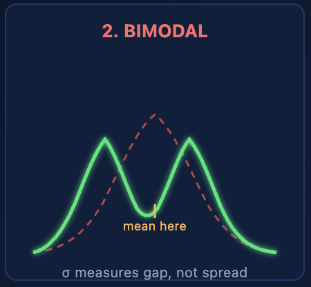 Two mold cavities producing slightly different dimensions. Day shift and night shift with different thermal conditions. Two raw material suppliers with different lot properties. When these sub-populations mix in your dataset, you get a bimodal distribution — two peaks with a valley between them.
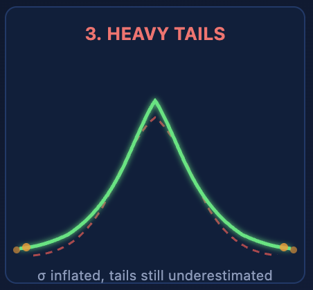 A normal distribution predicts that values beyond ±3σ occur 0.3% of the time — roughly 3 parts in 1,000. Many industrial processes produce outliers at rates of 1–5%, sometimes more. Measurement noise, transient equipment hiccups, contaminated raw material lots, and startup effects all generate occasional extreme values that a Gaussian tail doesn't account for.
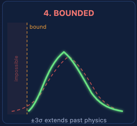 If your process measures a percentage (0–100%), a concentration (≥ 0), a surface roughness (≥ 0), or any physical quantity with hard limits, the ±3σ interval can extend into regions that are physically impossible. A concentration with mean = 2 ppm and σ = 1.5 ppm gives a lower 3σ limit of −2.5 ppm. Negative concentration doesn't exist.
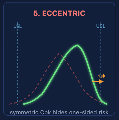 Tool wear causes a progressive drift during a production run. A process targets the low end of the spec window to maximize tool life. Asymmetric adjustment after changeover. All of these produce data where the mean sits off-center relative to the spec limits, and the distribution is asymmetric around that mean.