Every quality engineer trusts Cpk — but the Cpk normality assumption behind it rarely holds. The ±1σ covers 68%, ±3σ covers 99.7% rule only works if your data follows a perfect Gaussian bell curve. In real manufacturing, it almost never does.
So what happens when you build your entire capability reporting on an assumption that doesn't hold? Let's find out.
How to Test the Cpk Normality Assumption in 30 Seconds
Take any production dataset you're currently reporting Cpk on — 50 to 200 measurements of a critical dimension — and run a Kolmogorov-Smirnov test against a normal distribution. Compare the empirical CDF of your actual data to the theoretical Gaussian CDF.
The mathematical proof that your Cpk is wrong: Kolmogorov–Smirnov convergence, Chebyshev’s inequality, and why σ-based intervals fail when the empirical CDF diverges from the Gaussian hypothesis. A master’s-level walkthrough of what the Cpk normality assumption actually assumes — and where it breaks
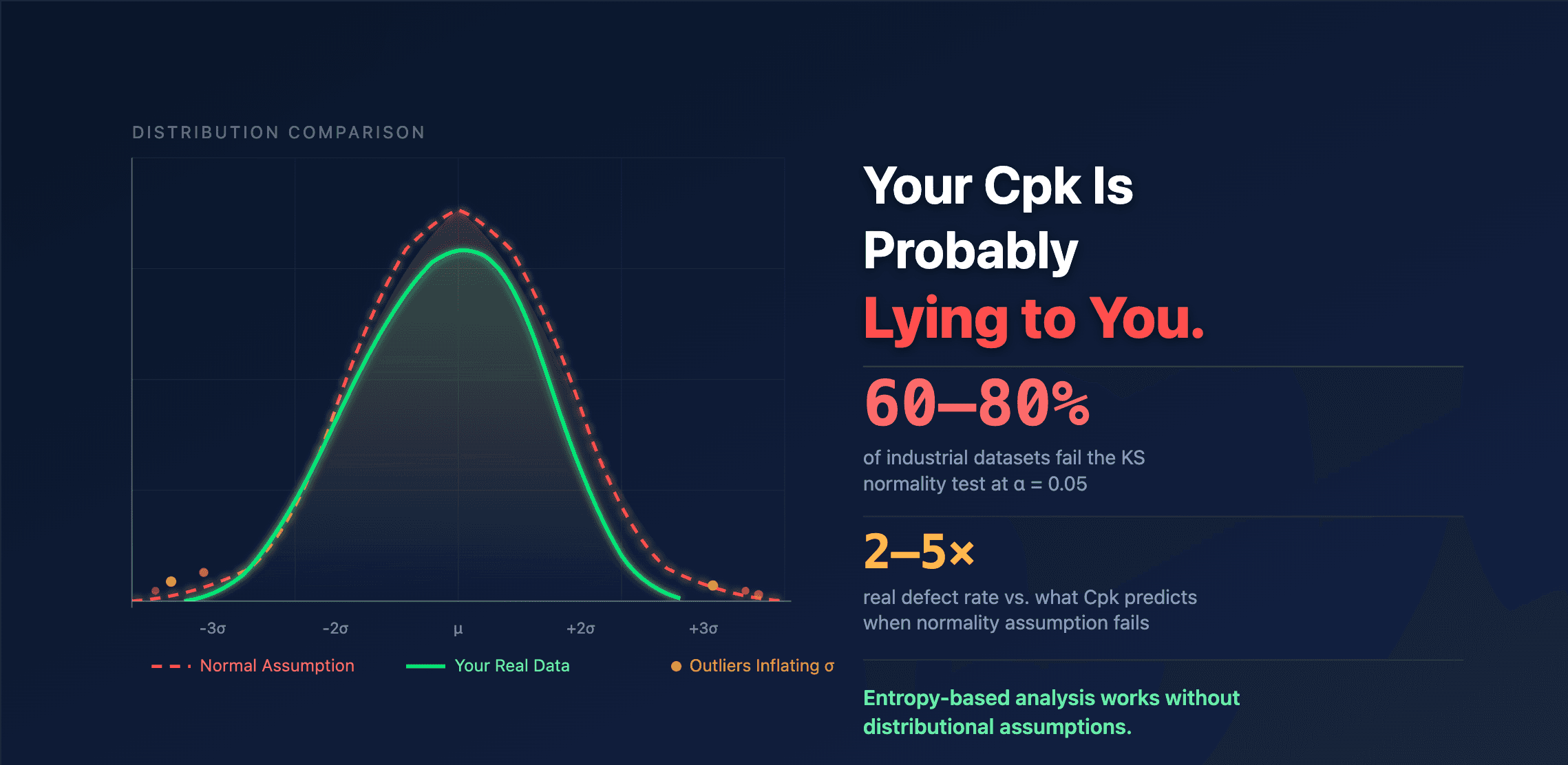
The result? In practice, 60–80% of industrial datasets fail the normality test at α = 0.05. The p-values aren't borderline — they often drop below 0.01. With larger samples from inline measurement systems (500+ points), rejection rates climb above 90%.
Your data isn't normal. Your Cpk assumes it is. That gap has a cost.
Why Industrial Data Breaks the Normality Assumption
This isn't bad luck or bad measurement — it's physics and process reality:
Tool wear and drift mean the first part and the last part in a run come from slightly different distributions. Pool them together and you get a flat-topped shape that looks bell-curved on a histogram but fails every formal test.
Multiple variation sources — different cavities, fixtures, operators, raw material lots — each contribute a slightly shifted sub-population. The mixture looks roughly Gaussian to the eye. It isn't.
Physical bounds create inherent skewness. Concentrations can't go negative. Surface roughness has hard limits. A dimension machined near a physical stop will always have a one-sided tail.
Inspection truncation removes the extremes. If you sort out-of-spec parts before analysis, your remaining data is truncated — which, by definition, is not normal.
Every one of these is structural and permanent. No amount of "better measurement" will make industrial data Gaussian. The Cpk normality assumption is fighting physics.
What a Broken Cpk Normality Assumption Actually Costs You
When σ is inflated by outliers, mixed populations, or non-normality, the consequences are concrete:
A process that looks like Cpk = 0.9 (not capable — invest $500K in improvement) might actually be running at true capability of 2.1 (highly capable — the "variation" was data contamination, not process instability). Conversely, a comfortable-looking Cpk = 1.45 might be masking a real defect rate 3–5× higher than what the normality assumption predicts. Your scrap logs know the truth. Your Cpk report doesn't.
The Industry's Workarounds — and Their Limits
Quality teams aren't blind to the Cpk normality assumption problem. But the standard responses each have significant drawbacks:
Ignore it — the most common approach. Calculate Cpk anyway, submit it in the PPAP, and maintain a polite fiction with the customer. It works until your warranty costs don't match your capability reports.
Transform the data — Box-Cox or Johnson transformations force data into something normal-ish. But now your control limits live in transformed space. Try explaining to a production manager what a limit of 2.37 in Johnson SB space means in actual millimeters.
Fit a different distribution — Weibull, log-normal, beta. Better in theory, but with small samples, multiple distributions fit equally well while giving very different tail probabilities. And the tails are exactly where your out-of-spec risk lives.
Beyond the Cpk Normality Assumption: Distribution-Free Methods
Instead of forcing your data into a distributional assumption, ask the opposite question: What does the data itself tell you about your process?
Entropy-based statistical methods work directly with the empirical distribution — no normality assumption, no distribution selection, no transformation. They separate genuine process variation from noise, outliers, and data contamination automatically.
The practical difference: when you compare the predicted defect rate from a normality-based Cpk against the predicted rate from distribution-free entropy analysis, and then check both against your actual scrap records — the entropy-based estimate matches reality. Consistently.
That's not a methodology debate. That's a business result.
The Takeaway
Run the Kolmogorov-Smirnov test on your own data today. If it rejects the normality assumption — and it very likely will — you now know that every sigma-based Cpk metric you're reporting carries an unquantified error. The question isn't whether to modernize your statistical toolkit. The question is how much the current gap between your reports and your reality is costing you.
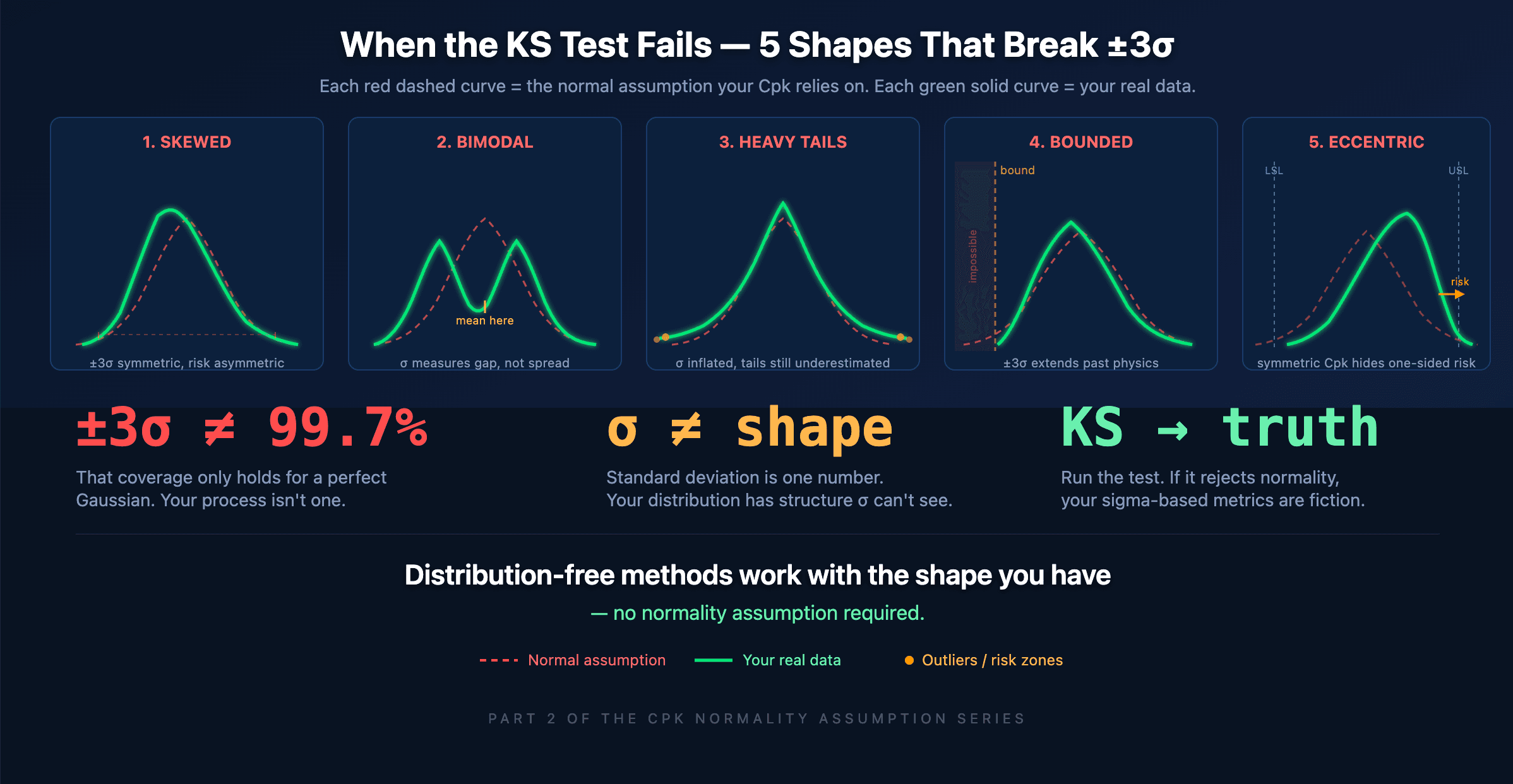
When a KS test rejects the Cpk normality assumption, the ±3σ interval stops meaning 99.7%. Here are five real process shapes where sigma-based reasoning falls apart — and what your data is actually telling you.