Your aggregate Cpk says 1.42. Your scrap logs say something else. Hidden clusters in your process data explain why — and Cpk can't see them.
Here's the scenario: 500 injection-molded parts from a four-cavity mold. Aggregate analysis shows Cpk = 1.42. Above the 1.33 threshold. Capable. Everyone signs off.
What is EGDF? The Entropic Global Distribution Function skips distribution fitting entirely — learning your process shape from the data. Here’s how EGDF and ELDF work, when they outperform traditional methods, and why they produce reliable Cpk from small samples.
But behind that 1.42 are four cavities running at four different means. Cavity 1 and 3 are tight — Cpk above 1.8. Cavity 4 is marginal at 1.15. Cavity 2 is at 0.87. Non-capable. Producing defects on every run.
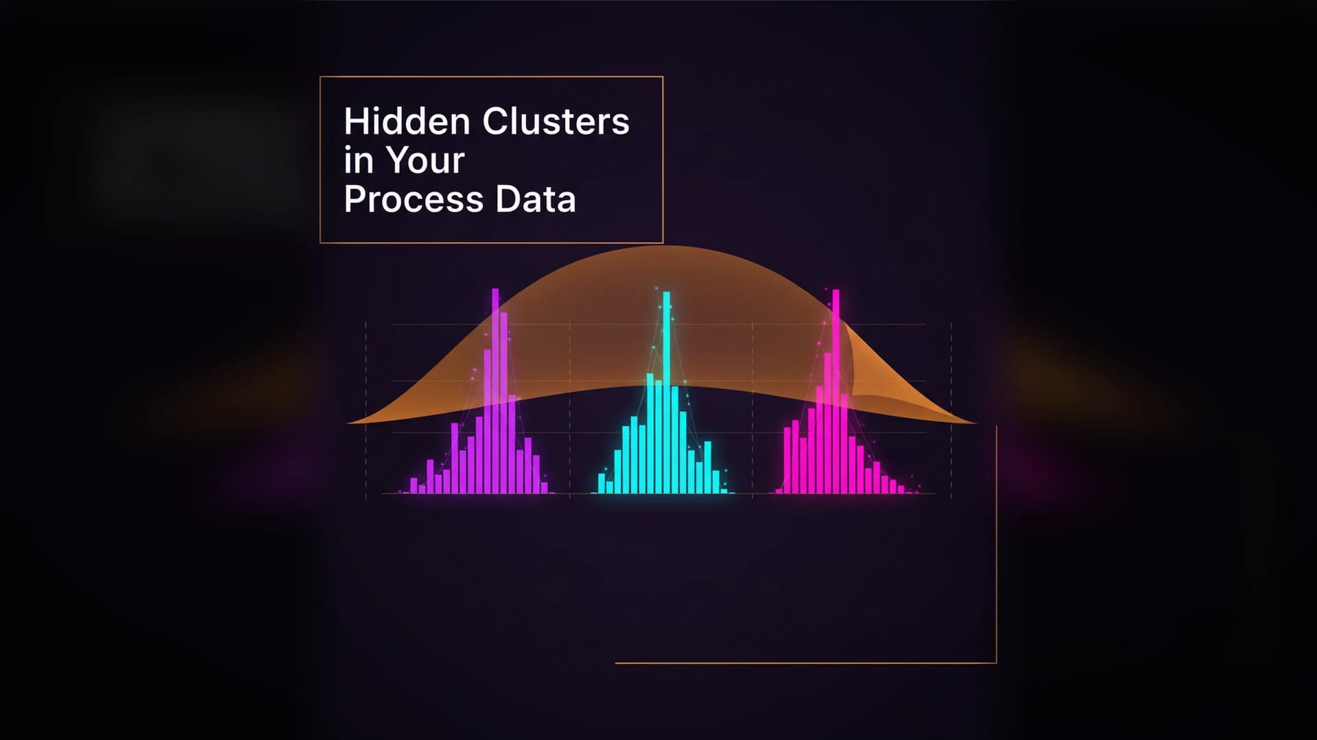
The aggregate Cpk hid the problem because cavities 1 and 3 pulled the average up. The data looked like one wide distribution. It was actually four narrow ones stacked on top of each other.
Why Cpk Can't See Clusters
Traditional capability analysis makes an assumption so fundamental that nobody mentions it: the data comes from a single process. One mean. One standard deviation. One distribution.
When that assumption holds, Cpk works exactly as intended. When it doesn't — when the data contains hidden subpopulations from multiple sources — Cpk computes a single number that describes none of the actual processes.
Consider what happens mathematically. Two clusters with different means produce a pooled standard deviation larger than either individual σ. That inflated σ enters the Cpk denominator. The result: a capability index that's worse than the best cluster and better than the worst cluster. The aggregate number is optimistic about the bad cavities and pessimistic about the good ones.
Neither reading is useful. The aggregate Cpk answers a question nobody asked: "what's the capability if you pretend all these different processes are one?"
Where Hidden Clusters Come From
Manufacturing processes create subpopulations constantly. The sources are mundane and everywhere:
Multi-cavity molds. Each cavity has slightly different dimensions, cooling rates, and flow characteristics. Four cavities, four means. Pool them and the histogram shows a wide, flat-topped shape that isn't any named distribution.
Tool wear across a production run. The first part and the last part come from effectively different processes. Tool wear creates a systematic drift that, when measured in aggregate, looks like a non-normal distribution with heavy tails. It's not heavy tails — it's two process states blended together.
Shift-to-shift variation. Day crew and night crew set up differently. Different operators, different habits, slightly different fixture torques. Two shifts, two distributions, one capability report.
Material lots. Batch-to-batch variation in raw material properties creates subpopulations that persist through the process. Lot A runs 2μm tighter than Lot B. Mix them in the capability study and the variance doubles.
Parallel machines or stations. Multiple CNC machines running the same part number at slightly different calibrations. Slightly different means. Identical part numbers. One data stream.
Every one of these scenarios produces data that looks like one distribution but is actually several. And every one is invisible to traditional Cpk.
The Business Cost of Invisible Clusters
Two real outcomes from hidden clusters:
The false-pass PPAP. Aggregate Cpk = 1.35. Above threshold. Customer accepts the submission. But one cavity or one machine is at 0.88. Defects from that source ship to the customer. Six months later, you're answering quality complaints about a "capable" process and launching corrective actions you can't explain — because the data said everything was fine.
The unnecessary process investment. Aggregate Cpk = 1.08. Below threshold. Engineering approves $200K for new tooling. But three of four cavities are at 1.5+. One cavity is at 0.75. The fix is a $5K cavity repair, not a $200K retool. Without cluster visibility, you can't distinguish "entire process is marginal" from "one source is bad."
Both scenarios cost money. The first costs customer trust. The second costs capital. Neither would happen if the analysis could see the clusters.
How ELDF Detects What Cpk Hides
The Entropic Local Distribution Function (ELDF) analyzes data density at a local level, using information entropy to identify where subpopulations exist.
Traditional cluster detection methods — k-means, Gaussian mixture models — require you to specify how many clusters to look for. That's a guess. Specify 2 and you'll find 2 even if there are 4. Specify 4 and you'll split a genuine single process into artificial subgroups.
ELDF discovers clusters from the data's entropy structure. Regions of high local density separated by regions of low density indicate distinct subpopulations. The method doesn't ask how many clusters exist. It finds them.
The workflow:
Homogeneity testing first: is this data from a single process or multiple? A clear yes/no answer before any decomposition.
If non-homogeneous: ELDF decomposes the data into subpopulations, each with its own distribution function and capability index.
Per-cluster Cpk: Instead of one number that describes nothing, you get specific numbers for each source. Cavity 1: 1.85. Cavity 2: 0.87. Cavity 3: 1.72. Cavity 4: 1.15.
Now you know exactly where the problem is. Not "the process is marginal." Instead: "Cavity 2 needs maintenance."
The Homogeneity Question Nobody Asks
Before you compute any capability index — traditional or entropy-based — the first question should be: is this data homogeneous?
If the answer is no, a single Cpk is meaningless regardless of the method. You can compute the most mathematically sophisticated capability index in existence, and if the data contains hidden clusters, the result is still a fiction.
Subgroup analysis in traditional SPC addresses this partially — rational subgrouping separates known sources (shifts, machines, lots). But it requires you to know the sources in advance and tag each measurement accordingly. Hidden clusters are hidden precisely because the source isn't known or recorded.
That's the gap ELDF fills: detecting subpopulations that exist in the data but aren't captured in the metadata. The clusters you didn't know to look for.
Five Signs Your Data Has Hidden Clusters
Before running formal analysis, these patterns in your data suggest subpopulations:
Flat-topped histogram. A normal distribution has a single peak. A flat top suggests two or more overlapping distributions with different means. The wider the flat region, the more separated the clusters.
Cpk and Ppk disagree significantly. When Ppk (computed from overall σ) is much lower than Cpk (computed from within-subgroup σ), there's substantial between-subgroup variation. That variation may come from hidden clusters.
Bimodal or multimodal shape. The most obvious signal — two or more peaks in the histogram. But subtle bimodality with closely spaced means can look like a single wide peak.
Non-normality that doesn't fit any distribution. You run goodness-of-fit tests against Weibull, lognormal, gamma — nothing fits well. The data isn't any named distribution because it's a mixture of simpler distributions.
Scrap that doesn't match capability. High Cpk but persistent low-level scrap. The aggregate says "capable" but defects keep appearing. A cluster below the capability threshold can hide inside an otherwise healthy dataset.
Stop Averaging. Start Decomposing.
Your process data is trying to tell you something specific. Aggregate Cpk compresses that information into one number — and loses the signal in the compression.
Hidden clusters aren't rare. They're the natural consequence of manufacturing complexity. Multiple cavities, multiple shifts, multiple lots, multiple machines. The question isn't whether clusters exist in your data. The question is whether your analysis can find them.
Upload your process data and see if hidden clusters are affecting your capability numbers — homogeneity testing and per-cluster Cpk in under 60 seconds. Analyze your data free →
Process drift hides under false alarms. Shewhart charts catch sudden shifts but miss gradual process drift — while Nelson rules fire on stable data. Entropy-based homogeneity testing separates real drift from noise without chart configuration.