You tested for normality. It failed. Now what — fit a Weibull? A lognormal? What if EGDF could skip the guessing entirely?
The textbook answer is "fit a different distribution" — pick from a menu of Weibull, lognormal, beta, or gamma, estimate parameters, and hope the tails behave. But with 15 measurements from a prototype run, three of those distributions pass the goodness-of-fit test while giving Cpk estimates that range from 0.89 to 1.51. Which one is right?
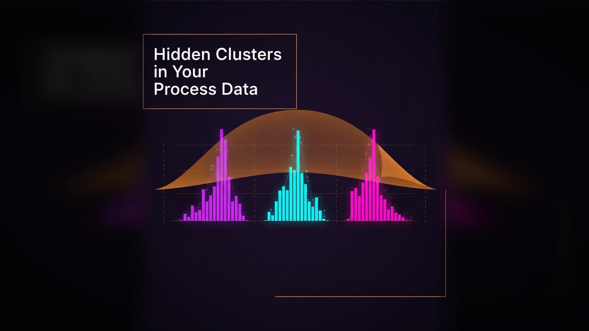
Hidden clusters from multi-cavity molds, shift changes, and material lots produce aggregate Cpk that looks capable — while one subpopulation ships defects. ELDF detects what Cpk can’t see.
None of them. The question itself is wrong. You don't need to name your distribution. You need to measure it.
Why Distribution Guessing Fails (and How EGDF Solves It)
Traditional SPC follows a rigid workflow:
Collect measurements
Assume (or test for) normality
Estimate mean and standard deviation
Compute Cpk from those parameters
Step 2 fails for 60–80% of industrial data. So you go to Step 2b: guess a different distribution. But here's the problem nobody mentions — with small samples, you can't reliably distinguish between a Weibull, a lognormal, and a truncated normal. They all produce acceptable p-values. They all give different tail probabilities. And the tails are where your scrap lives.
Distribution fitting replaces the normality assumption with a different assumption — and calls it a solution.
What If You Didn't Have to Guess?
The Entropic Global Distribution Function (EGDF) skips the guessing entirely. Instead of assuming your data follows a named distribution and estimating parameters, EGDF learns the actual shape of your process distribution directly from your measurements.
The intuition is simple: information entropy measures how much "surprise" each new data point carries. A tight, stable process has low entropy — each measurement is predictable. A scattered process has high entropy. EGDF uses this principle to build a smooth distribution function that captures whatever shape your data actually has — skew, heavy tails, bimodality, bounded ranges. All of it.
Three things make this different from traditional fitting:
No distribution selection. EGDF doesn't fit a Weibull. It doesn't fit a lognormal. It constructs a function faithful to your data's actual shape. If your data happens to be normal, EGDF will look Gaussian. If it's not, EGDF won't force it.
Stable with small samples. Traditional estimation of mean (μ) and standard deviation (σ) converges slowly — with 10 measurements, your σ estimate carries enormous uncertainty. EGDF doesn't estimate μ or σ at all. It builds the distribution function directly. The result: reliable capability indices with as few as 5–8 measurements, where traditional Cpk needs 30+ to stabilize.
Honest uncertainty. When the data doesn't support a conclusion, EGDF's entropy structure shows it. No false precision from an assumed parametric model.
The Hidden Problem Inside Your "Good" Cpk
If EGDF is the satellite view of your process, the Entropic Local Distribution Function (ELDF) is the microscope.
Here's a scenario that happens more than quality teams realize: your aggregate process capability shows Cpk = 1.35. Above the 1.33 threshold. Ship it.
But ELDF decomposes that dataset and finds two subpopulations:
Cluster A (60% of parts): Cpk = 1.85
Cluster B (40% of parts): Cpk = 0.88
Cluster B is producing defects. The aggregate Cpk hides this because Cluster A pulls the average up. Your PPAP says "capable." Your scrap logs say otherwise.
Where do hidden clusters come from?
Multi-cavity molds. Each cavity runs at a slightly different mean. Pooled data looks like one wide distribution. ELDF sees four tight ones.
Shift changes. Day and night crews set up differently. One distribution in the report. Two in reality.
Material lots. Batch-to-batch variation creates invisible subpopulations.
Parallel tool stations. Slightly different calibrations. Slightly different means. One blended Cpk.
Traditional cluster detection methods (k-means, GMM) force you to specify how many clusters to look for. ELDF discovers them automatically from the data's entropy structure.
How They Work Together
In practice, you never run EGDF or ELDF in isolation:
EGDF maps the global distribution — the overall shape of your process
ELDF (when non-homogeneous) decomposes into subpopulations with per-cluster capability indices
This replaces the traditional assumption-test-fit-report cycle with something more honest: measure what's actually there and report what's actually happening.
When the Gap Is Biggest
Entropy-based and traditional methods agree when data is genuinely normally distributed. That happens — additive measurement error, some chemical concentrations, certain thermal processes.
The results diverge sharply when:
Samples are small (n < 25): parametric σ estimate is unstable, EGDF holds steady
Data is non-normal: skewed, bounded, heavy-tailed, or multimodal — non-normal data is the norm in manufacturing
The number matters: PPAP submissions, customer audits, process qualification — where a wrong Cpk has dollar consequences
For assumption-free statistics, the principle is straightforward: let the data speak instead of making it conform.
Stop Guessing. Start Measuring.
If you've ever stared at a Cpk number and thought "this doesn't match what I see on the floor" — you were probably right. The gap wasn't your intuition. It was the normality assumption.
EGDF and ELDF close that gap. Not by choosing a better assumption, but by dropping the assumption entirely.
Upload your process data and see your actual distribution in under 60 seconds — no normality assumption, no distribution selection, no guesswork. Try EntropyStat free →
Minitab offers non-normal options. EntropyStat is distribution-free. Those aren’t the same thing. Offering a menu of distributions to choose from is distribution-flexible — not distribution-free. Here’s why that distinction determines whether your Cpk is correct.